Sensitivity analysis and design optimization

Author: Anne Disabato, Tim Hanrahan, Brian Merkle

Steward: David Chen, Fengqi You

Date Presented: February 23, 2014

Introduction

Optimization and sensitivity analysis are key aspects of successful process design. Optimizing a process maximizes project value and plant performance, minimizes project cost, and facilitates the selection of the best components [1].

Design Optimization

Economic optimization is the process of finding the condition that maximizes financial return or, conversely, minimizes expenses. The factors affecting the economic performance of the design include the types of processing technique and equipment used, arrangement, and sequencing of the processing equipment, and the actual physical parameters for the equipment. The operating conditions are also of prime concern.

Optimization of process design follows the general outline below:

1. Establish optimization criteria: using an objective function that is an economic performance measure.
2. Define optimization problem: establish various mathematical relations and limitations that describe the aspects of the design
3. Design a process model with appropriate cost and economic data

Although profitability or cost is generally the basis for optimization, practical and intangible factors usually need to be included as well in the final investment decision. Such factors are often difficult or impossible to quantify, and so decision maker judgment must weigh such factors in the final analysis [3], [4].

Defining the Optimization Problem and Objective Function

In optimization, we seek to maximize or minimize a quantity called the goodness of design or objective function, which can be written as a mathematical function of a finite number of variables called the decision variables.

$z=f(x_{1},x_{2},...x_{n})$

The decision variables may be independent or they may be related via constraint equations. Examples of process variables include operating conditions such as temperature and pressure, and equipment specifications such as the number of trays in a distillation column. The conventional name and strategy of this optimization method varies between texts; Turton suggests creating a base case prior to defining the objective function and Seider classifies the objective function as a piece of a nonlinear program (NLP) [5], [6].

A second type of process variable is the dependent variable; a group of variables influenced by process constraints. Common examples of process constraints include process operability limits, reaction chemical species dependence, and product purity and production rate. Towler & Sinnott define equality and inequality constraints [2]. Equality constraints are the laws of physics and chemistry, design equations, and mass/energy balances:

$h(x_{1},x_{2},...x_{n})=b_{1}$

For example, a distillation column that is modeled with stages assumed to be in phase equilibrium often has several hundred MESH (material balance, equilibrium, summation of mole fractions, and heat balance) equations. However, in the implementation of most simulators, these equations are solved for each process unit, given equipment parameters and steam variables. Hence, when using these simulators, the equality constraints for the process units are not shown explicitly in the nonlinear program. Given values for the design variables, the simulators call upon these subroutines to solve the appropriate equations and obtain the unknowns that are needed to perform the optimization [5].

Inequality constraints are technical, safety, and legal limits, economic and current market:

$g(x_{1},x_{2},...x_{n}){\frac {\geq }{\leq }}b_{2}$

Inequality constrains also pertain to equipment; for example, when operating a centrifugal pump, the head developed is inversely related to the throughput. Hence, as the flow rate is varied when optimizing the process, care must be taken to make sure that the required pressure increase does not exceed that available from the pump [5].

It is important that a problem is not under or over-constrained so a possible solution is attainable. A degree-of-freedom (DOF) analysis should be completed to simply the number of process variables, and determine if the system is properly specified.

Trade-Offs

A part of optimization is assessing trade-offs; usually getting better performance from equipment means higher cost. The objective function must capture this trade-off between cost and benefit.

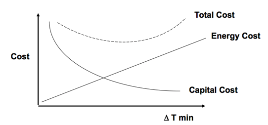
Example: Heat Recovery, total cost captures trade-off between energy savings and capital expense.

Figure 1: Trade-off example [1]

Some common design trade-offs are more separations equipment versus low product purity, more recycle costs versus increased feed use and increased waste, more heat recovery versus cheaper heat exchange system, and marketable by-product versus more plant expense.

Parametric Optimization

Parametric optimization deals with process operating variables and equipment design variables other than those strictly related to structural concerns. Some of the more obvious examples of such decisions are operating conditions, recycle ratios, and steam properties such as flow rates and compositions. Small changes in these conditions or equipment can have a diverse impact on the system, causing parametric optimization problems to contain hundreds of decision variables. It is therefore more efficient to analyze the more influential variables effect on the overall system. Done properly, a balance is struck between increased difficulty of high-variable-number optimization and optimization accuracy. [3]

Suboptimizations

Simultaneous optimization of the many parameters present in a chemical process design can be a daunting task due to the large number of variables that can be present in both integer and continuous form, the non-linearity of the property prediction relationships and performance models, and frequent ubiquity of recycle. It is therefore common to seek out suboptimizations for some of the variables, so as to reduce the dimensionality of the problem [3]. While optimizing sub-problems usually does not lead to overall optimum, there are instances for which it is valid in a practical, economic sense. Care must always be taken to ensure that subcomponents are not optimized at the expense of other parts of the plant.

Equipment optimization is usually treated as a subproblem that is solved after the main process variables such as reactors conversion, recycle ratios, and product recoveries have been optimized.

Optimization of a Single Decision Variable

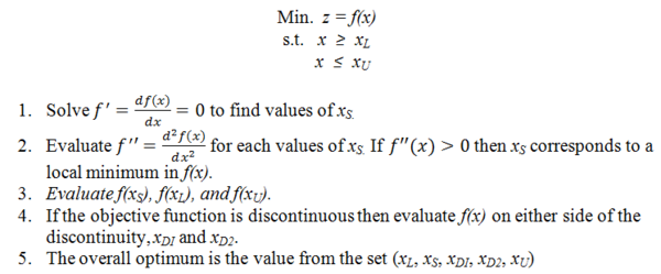
If the objective is a function of a single variable, x, the objective function f(x) can be differentiated with respect to x to give f’(x). The following algorithm summarizes the procedure:

Below is a graphical representation of the above algorithm.

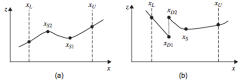
Figure 2. Graphical Illustration of (a) Continuous Objective Function (b) Discontinuous Objective Function

In Figure2a, $x_{L}$ is the optimum point, even though there is a local minimum at $x_{S}1$; In Figure 2b, the optimum is at $x_{D}I$.

Search Methods

Search methods are at the core of the solution algorithms for complex multivariable objective functions. The four main search functions are unrestricted search, three-point interval search, golden-section search, and quasi-newton method [1].

Unrestricted Search

Unrestricted Searching is a relatively simple method of bounding the optimum for problems that are not constrained. The first step is to determine a range in which the optimum lies by making an initial guess of x and assuming a step size, h. The direction of search that leads to improvement in the value of the objective is determined by z1, z2, and z3 where

$z_{1}=f(x)$

$z_{2}=f(x+h)$

$z_{3}=f(x-h)$

The value of x is then increased or decreased by successive steps of h until the optimum is passed. In engineering design problems it is almost always possible to state upper and lower bounds for every parameter, so unrestricted search methods are not widely used in design.

The three-point interval is done as follows:

1. Evaluate f(x) at the upper and lower bounds, $x_{L}$ and $x_{U}$, and at the center point, ${\frac {x_{L}+x_{U}}{2}}$.
2. Two new points are added in the midpoints between the bounds and the center point, at ${\frac {3x_{L}+x_{U}}{4}}$ and ${\frac {x_{L}+3x_{U}}{4}}$
3. The three adjacent points with the lowest values of f(x) (or the highest values for a maximization problem) are then used to define the next search range.

By eliminating two of the four quarters of the range at each step, this procedure reduces the range by half each cycle. To reduce the range to a fraction ε of the initial range therefore takes n cycles, where $\epsilon =0.5^{n}$. Since each cycle requires calculating f (x) for two additional points, the total number of calculations is $2n={\frac {2log\epsilon }{log0.5}}$. The procedure is terminated when the range has been reduced sufficiently to give the desired precision in the optimum. For design problems it is usually not necessary to specify the optimal value of the decision variables to high precision, so $\epsilon$ is usually not a very small number.

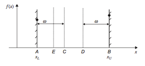
The golden-section search is more computationally efficient than the three-point interval method if $\epsilon <0.29$. In the golden-section search only one new point is added at each cycle. The golden-section method is illustrated in Figure 3.

Figure 3: Golden-Section Method

We start by evaluating $f(x_{L})$ and $f(x_{U})$ corresponding to the upper and lower bounds of the range, labeled A and B in the figure. We then add two new points, labeled C and D, each located a distance ωAB from the bounds A and B, i.e., located at

and

For a minimization problem, the point that gives the highest value of f(x) is eliminated. In Figure 3, this is point B. A single new point, E, is added, such that the new set of points AECD is symmetric with the old set of points ACDB. For the new set of points to be symmetric with the old set of points,

$AE=CD=$ω$AD$

But we know

$DB=$ω$AB$

so

$AD=(1-$ω$)AB$

$CD=(1-2$ω$)AB$

$(1-2$ω$)=$ω$(1-$ω$)$

${\displaystyle }$ω$={\frac {(3\pm {\sqrt {5}})}{2}}$

Each new point reduces the range to a fraction 1 − ω = 0.618 of the original range. To reduce the range to a fraction $\epsilon$ of the initial range therefore requires $n={\frac {log\epsilon }{log0.618}}$ function evaluations. The number 1 − ω is known as the golden mean.

The Quasi-Newton method is a super-linear search method that seeks the optimum by solving f’(x) and f’’(x) and searching for where f’(x) = 0. The value of x at step k + 1 is calculated from the value of x at k using

$x_{(}k+1)=x_{k}-{\frac {f'(x_{k})}{f''(x_{k})}}$

and the procedure is repeated until $(xk+1-xk)$ is less than a convergence tolerance, $\epsilon$. If we do not have explicit formulate for f’(x) and f’’(x), then we can make a finite difference approximation about a point:

$x_{(}k+1)=x_{k}-{\frac {\frac {f(x_{k}+h)-f(x_{k}-h)}{2h}}{(f(x_{k}+h)-2f(x)+{\frac {f(x_{k}-h)}{h^{2}}})}}$

The Quasi-Newton method generally gives fast convergence unless f’’(x) is close to zero, in which convergence is poor.

All of the methods discussed in this section are best suited for unimodal functions, functions with no more than one maximum or minimum within the bounded range.